Modelling for count responses

ANU BDSI
workshop
Generalised Linear Models

Emi Tanaka

Biological Data Science Institute

27th September 2024

Case study: Abundance of Noisy Miners

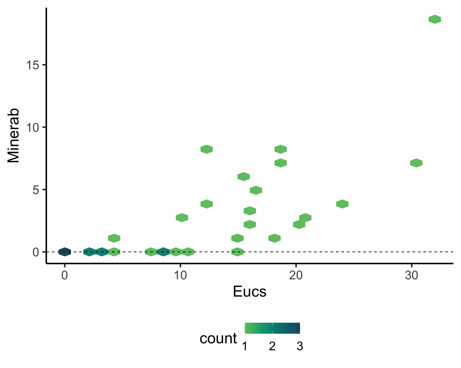
  • The noisy miner is a small but aggressive native Australian bird.
  • A study of the habitats of the noisy miner recorded the abundance of noise miners in two hectare transects located in buloke woodland patches along its characteristics,
    • Eucs = number of eucalypt trees, and
    • Minerab = abundance of noisy miners.
Code
data(nminer, package = "GLMsData")
base <- nminer |> 
  ggplot(aes(Eucs, Minerab)) +
  geom_hex() +
  colorspace::scale_fill_continuous_sequential(breaks = 1:3, palette = "ag_GrnYl", begin = 0.3) +
  geom_hline(yintercept = 0, linetype = 2) +
  theme(legend.position = "bottom")

base

Linear regression

Code
base + 
  geom_smooth(method = lm, se = FALSE, linewidth = 2) +
  labs(title = "lm(Minerab ~ Eucs)") +
  guides(fill = "none")

Code
base +
  geom_smooth(method = lm, se = FALSE, linewidth = 2, 
              formula = sqrt(y) ~ x, 
              aes(y = stage(Minerab, after_stat = y^2))) +
  labs(title = "lm(sqrt(Minerab) ~ Eucs)") +
  guides(fill = "none")

Code
base +
  geom_smooth(method = lm, se = FALSE, linewidth = 2) +
  scale_y_sqrt() +
  labs(title = "lm(sqrt(Minerab) ~ Eucs)") +
  guides(fill = "none")

  • Negative values for abundance are not possible.
  • The count of noisy miners does not have a known restrictive count for using Binomial distribution.

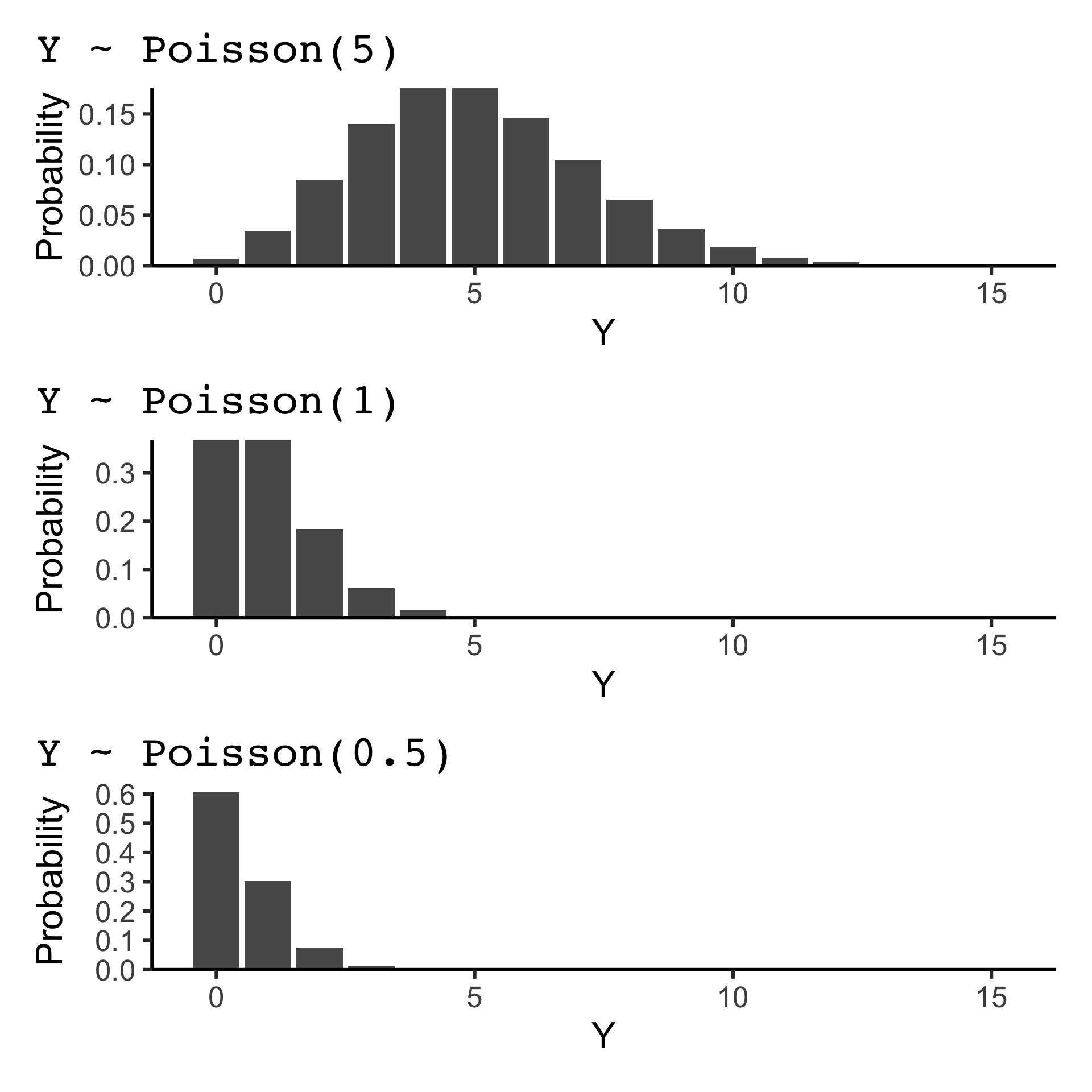
Poisson distribution

  • If Y \sim \text{Poisson}(\lambda), then P(Y = y) = \frac{e^{-\lambda} \lambda^y}{y!} for y = 0, 1, 2, \ldots and \lambda > 0.

  • The mean and variance of Y are both \lambda.

  • The Poisson distribution is often used to model (unrestricted) count data.

Poisson regression model

  • We assume Y_i \sim \text{Poisson}(\mu_i) and model the mean \mu_i as:

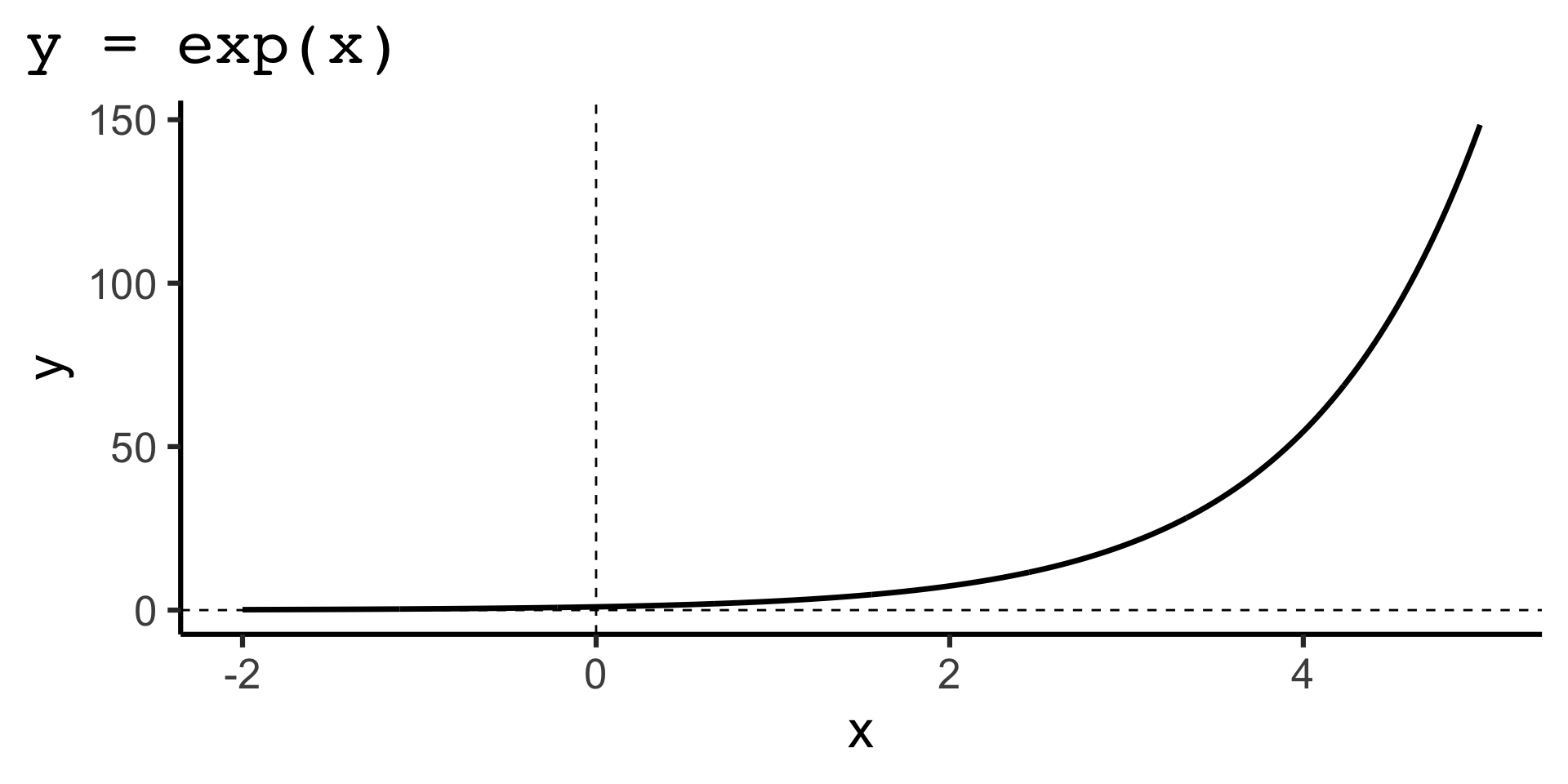
\log_e(\mu_i) = \beta_0 + \beta_1x_{i1} + \beta_1x_{i2} + \ldots + \beta_kx_{ik}.
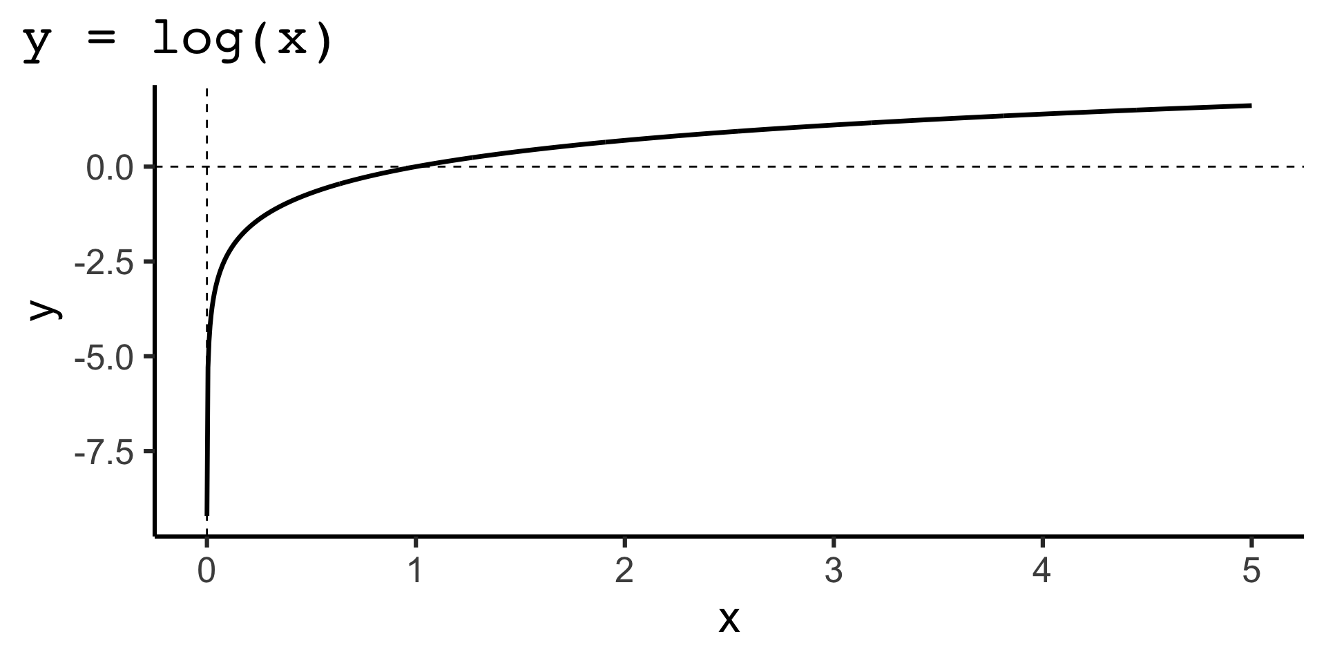
  • Then \hat{\mu}_i = \text{exp}(\hat{\beta}_0 + \hat{\beta}_1x_{i1} + \hat{\beta}_1x_{i2} + \ldots + \hat{\beta}_kx_{ik}).

Modelling counts with Poisson regression

Code
base + 
  geom_smooth(method = "glm", se = FALSE, linewidth = 2,
              method.args = list(family = poisson(link = "log"))) +
  geom_point(aes(y = .fitted), color = "red", size = 5,
             data = broom::augment(fit_glm, 
                 type.predict = "response",
                 newdata = tibble(Eucs = seq(0, 30, by = 10)))) +
  guides(fill = "none") +
  labs(title = "glm(Minerab ~ Eucs, \n    family = poisson(link = 'log'))") 
  • Predicting the response:

Case study: attitude to genetically modified foods

Code
gmfood <- read_csv("https://anu-bdsi.github.io/workshop-GLM/data/gmfood.csv")
Income Attitude Total
For Against
High 263 151 414
Low 258 222 480
Total 521 373 894
  • The data, collected between December 1996 and January 1997, includes the counts of the attitude (Against or For) of Australians to genetically modified foods according to their income (High or Low).
  • This data is presented often as a contingency table on left.

\chi^2 test for independence

H_0: p_{ij} = p_{i\cdot}p_{\cdot j}

Observed:

Expected:

  • \chi^2 = \dfrac{(\text{observed} - \text{expected})^2}{\text{expected}}
  • p-value = P(\chi^2_1 \geq \chi^2)

Poisson regression for contingency tables

  • Compare expected value under H_0 (independence) to no interaction in fit_main:
  • p-value for interaction effect is closely related to p-value from \chi^2 test for independence:

Main effects fix marginal totals

Income Attitude Total
For Against
High 263 151 414
Low 258 222 480
Total 521 373 894

Case study: cancer diagnosis

  • Types of cancer diagnosed in Western Australia in 1996 were recorded for males and females.
  • Females cannot have prostate cancer, and males cannot have cervical cancer.
  • Breast cancer is a possible, but very rare, disease among men
  • Note that a woman cannot get prostate cancer and a man cannot get cervix cancer.
  • A man can get breast cancer, but it is extremely rare.

Structural zeroes

  • Structural zeros need to be removed from the data.

Case study: Lung cancer in Danish cities

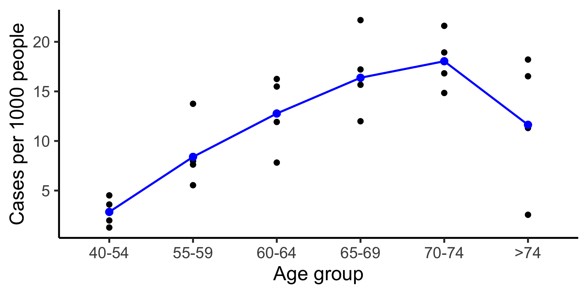
  • Number of incidents (out of the population) of lung cancer from 1968 to 1971 in four Danish cities recorded by age group.
Code
data(danishlc, package = "GLMsData")

danishlc |> 
  mutate(Age = fct_reorder(Age, parse_number(as.character(Age)), min)) |> 
  ggplot(aes(Age, Cases/Pop * 1000, color = City)) + 
  geom_point(size = 3) +
  geom_line(aes(group = City), linewidth = 1.2) +
  geom_text(aes(label = City), 
            hjust = 0, nudge_x = 0.1,
            data = ~filter(., Age == ">74"), size = 9) +
  guides(color = "none") +
  labs(y = "Cases per 1000 people", x = "Age group") +
  scale_x_discrete(expand = expansion(mult = c(0.1, 0.3)))

Modelling rates with Poisson regression

\log\left(\frac{\mu_i}{\texttt{Pop}_i}\right) = \beta_0 + \beta_{1\texttt{Age}_i} + \beta_{2\texttt{City}_i} + \beta_{3\texttt{AgeCity}_i}

\log(\mu_i) = \log(\texttt{Pop}_i) + \beta_0 + \beta_{1\texttt{Age}_i} + \beta_{2\texttt{City}_i} + \beta_{3\texttt{AgeCity}_i}

Chi-square test

  • We retain only Age in the model.

Predicting rate response with Poisson regression

Code
broom::augment(fit_glm3, type.predict = "response") |> 
  mutate(Pop = exp(`offset(log(Pop))`)) |> 
  mutate(Age = fct_reorder(Age, parse_number(as.character(Age)), min)) |> 
  ggplot(aes(Age, Cases/Pop * 1000)) +
  geom_point(size = 3) +
  geom_point(aes(y = .fitted/Pop * 1000), color = "blue", size = 4) +
  geom_line(aes(y = .fitted/Pop * 1000), color = "blue", group = 1, linewidth = 1.2) +
  labs(y = "Cases per 1000 people", x = "Age group") 
Case study: pock

Code
data(pock, package = "GLMsData")
ggplot(pock, aes(Dilution, Count)) +
  ggbeeswarm::geom_quasirandom(width = 0.2) +
  scale_x_continuous(transform = "log2")

  • In an experiment to assess viral activity, pock marks were counted at various dilutions of the viral medium.

Overdispersion

  • For a Poisson distribution, the variance should be equal to the mean.
Code
pock_group |>
  ggplot(aes(mean, var)) + 
  geom_point(size =3) +
  geom_smooth(method = lm, se = FALSE) + 
  geom_abline(intercept = 0, slope = 1, linetype = 2) + 
  scale_y_log10() +
  scale_x_log10() +
  labs(x = "Group mean", y = "Group variance")

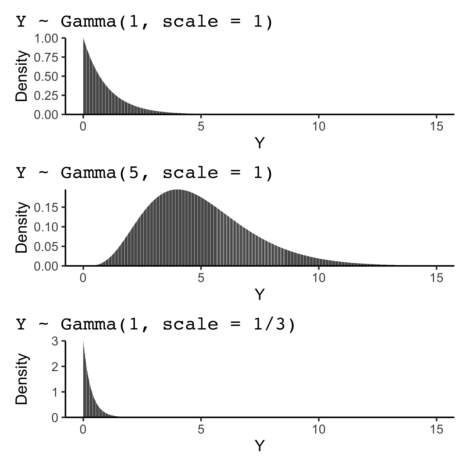
Gamma distrbution

Suppose Y \sim \text{Gamma}(k, \theta)

f(y) = \frac{1}{\Gamma(k)\theta^k}y^{k-1}e^{-y/\theta}

E(Y) = k\theta and var(Y) = k\theta^2
Negative binomial distribution

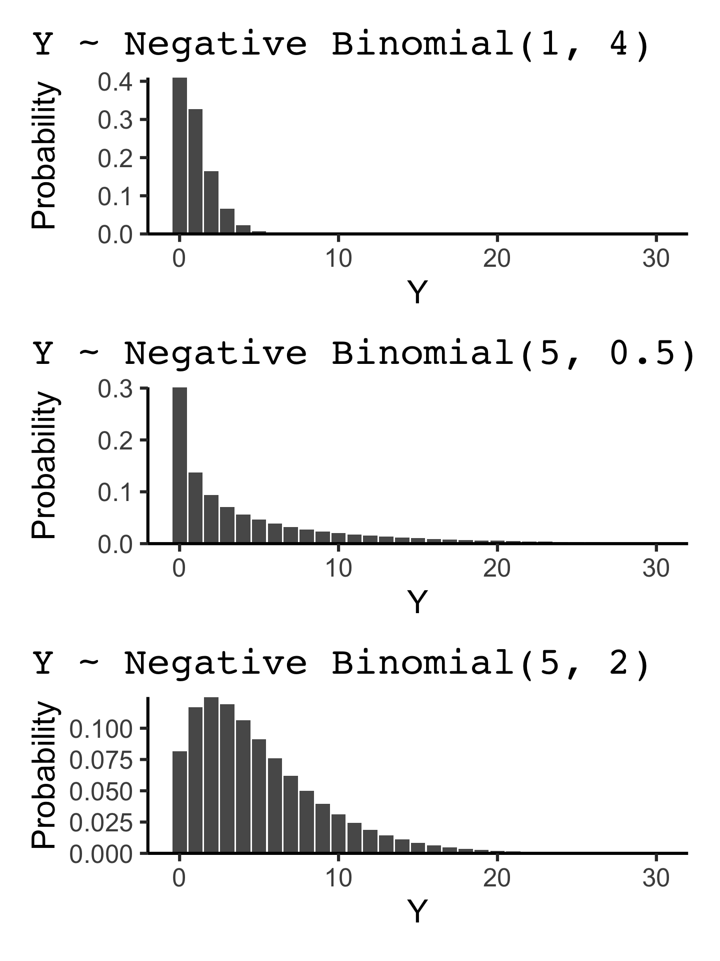
Y \sim \text{Negative Binomial}(m, k)

P(Y = y) = \frac{\Gamma(y + k)}{\Gamma(y + 1) \Gamma(k)} \left(\frac{m}{m + k}\right)^{y} \left(\frac{k}{m + k}\right)^{k}

where m is the mean and k is the inverse of the dispersion parameter.

E(Y) = m and \text{Var}(Y) = m + \frac{1}{r}m^2

Negative binomial regression

  • Suppose we consider a hierarchical model.
  • Instead of assuming Y_i \sim \text{Poisson}(\mu_i), we assume that:
    1. \lambda_i \sim \text{Gamma}(\mu_i, \psi).
    2. Y_i \sim \text{Poisson}(\lambda_i)
  • This hierarchical model in facts results in Y_i \sim \text{Negative Binomial}(\mu_i, k) where k = \frac{1}{\psi}.
  • E(Y_i) = \mu_i and \text{Var}(Y_i) = \mu_i + \psi \mu_i^2
  • If \psi = 0 then Negative Binomial reduces to Poisson.

Negative binomial regression in R

  • Negative binomial regression can be fitted using MASS::glm.nb() function:
  • The estimate of k is stored as theta in the model object:

Summary

  • You can model (unrestricted) count or rate data with Poisson regression using
    glm(y ~ x, family = poisson())
  • For rate data with the total size,
    glm(y ~ offset(log(size)) + x, family = poisson())
  • If the data is overdispersed (variance > mean), you can use Negative Binomial regression.
    MASS::glm.nb(y ~ x).